- Research
- Open access
- Published:
Deep learning enables parallel camera with enhanced- resolution and computational zoom imaging
PhotoniX volume 4, Article number: 17 (2023)
Abstract
High performance imaging in parallel cameras is a worldwide challenge in computational optics studies. However, the existing solutions are suffering from a fundamental contradiction between the field of view (FOV), resolution and bandwidth, in which system speed and FOV decrease as system scale increases. Inspired by the compound eyes of mantis shrimp and zoom cameras, here we break these bottlenecks by proposing a deep learning-based parallel (DLBP) camera, with an 8-μrad instantaneous FOV and 4 × computational zoom at 30 frames per second. Using the DLBP camera, the snapshot of 30-MPs images is captured at 30 fps, leading to orders-of-magnitude reductions in system complexity and costs. Instead of directly capturing photography with large scale, our interactive-zoom platform operates to enhance resolution using deep learning. The proposed end-to-end model mainly consists of multiple convolution layers, attention layers and deconvolution layer, which preserves more detailed information that the image reconstructs in real time compared with the famous super-resolution methods, and it can be applied to any similar system without any modification. Benefiting from computational zoom without any additional drive and optical component, the DLBP camera provides unprecedented-competitive advantages in improving zoom response time (~ 100 ×) over the comparison systems. Herein, with the experimental system described in this work, the DLBP camera provides a novel strategy to solve the inherent contradiction among FOV, resolution and bandwidth.
Introduction
Vision plays the most important role in information acquisition [1], and camera which is the most important mean besides the human eyes is essential for the acquisition of visual information. Camera researchers are faced with significant challenges of how to effectively achieve high-performance imaging [2,3,4,5,6,7,8,9,10,11,12,13,14,15], including wide-field high-resolution imaging [2, 5], high frame-rate imaging [10], and high dynamic range imaging [12]. A significant strategy that is used in cameras is to build a bridge between the parallel cameras and the wide-field-of-view (FOV) high-resolution imaging. Unfortunately, natural/artificial compound eyes [16,17,18,19,20,21,22,23,24] are suffering from a short line of sight and small numerical aperture that result in low spatial resolution. A study has also illustrated that if the spatial resolution of compound eye increases to the same level as the human’s eye, the radius of the whole lens is supposed to be at least 1 m [25]. Fortunately, facing the real-world scenery reconstruction tasks, array cameras [26,27,28,29,30] pave the way for smarter and more advanced imaging. Pan-and-scan panoramic techniques are initially used in wide-FOV imaging [31], but the extension of this method may only be feasible at extremely low frame rates (e. g. GigaPan Time Machine [32]). As a typical example, LSST [33] has a single optical lens, but uses 189 scientific sensors to capture an image with 3.2 GPs. As such, benefiting from multiscale design, David’s AWARE-2 [2], AWARE 10 [34] and AWARE 40 [3] cameras have already driven a transition from small-scale to large-scale spatial sampling. As an example, AWARE-2 uses 98 cameras to improve the data throughput and spatial resolution at three frames per minute. Moreover, the improved RUSH [5] with 35 CMOSs and modular hierarchical array camera [28] with 20 cameras, are no longer limited by the large overlapping-FOV. Researchers in Stanford University [10] have achieved remarkable results in cost control, including utilizing cheap cameras to build the system, and 4 large-PC platforms are also required to operate at the same time. More recently, mantis camera [4] with 18 cameras has simplified the complexity, but a relatively large and expensive electronic system is still required. In a word, the existing systems still follow the principle of digital zoom systems with high pixel count and high cost. Computational imaging may transform the central challenge of photography from the question of where to point the camera to that of how to achieve higher-performance imaging. Thus, if there is exactly a feasible solution to the above problems, the optical zoom obviously becomes an inexpensive and convenient answer. Understanding the direct transformation from digital zoom with high pixel count to optical zoom in parallel cameras has been a long-standing challenge with great scientific and practical importance. Optical zoom that magnifies details without changing the back working distance is very desirable for improving the imaging capability. Nowadays the existing optical zoom systems [35, 36] usually utilize the mechanical movement of multiple solid optical elements to amplify high-resolution details, at a speed of a few seconds. Adaptive lenses, such as elastomeric membrane lenses [37, 38], electrowetting lenses [39,40,41], and liquid crystal lenses [42,43,44], can be used for building optofluidic zooming systems [45,46,47,48]. However, the disadvantage for the above-mentioned existing systems necessitates an extended axial dimension as well as complex driving systems. The existing zoom systems can only magnify the central area of FOV and are incapable of magnifying the detail in marginal FOV. Herein, one of the key problems is how we can make the optical zoom in marginal FOV possible for parallel cameras. How exactly we can deal with the problems with a convenient and effective way has become a crucial challenge. Such a system, to the best of our knowledge, has never been achieved.
Here we propose a deep learning-based parallel camera with 4 × computational zoom that learns optical zoom, with an 8-μrad instantaneous FOV (IFOV) and 33-ms zoom speed, which uses 6 cameras to capture snapshot, 30-MPs images at 30 frames per second (fps). In this study, we have abandoned the high-pixel mode relying on a number of subarrays, and find a new way to replace the above method with an economical deep-learning model, which has competitive advantages over the existing zoom systems. Considerately, existing challenges are how array cameras can realize the zoom operation of any local area in the whole stitched FOV, especially the marginal FOV in each camera. We know yet no array camera can meet this standard, making optical zoom in marginal FOV possible. Hence, we present an end-to-end model, calculating ideal function from short-focus imaging to long-focus imaging over a stitched FOV, which dramatically reduces the number and complexity of subarrays. Benefiting from deep learning, the innovation is that both the array camera itself and the electronic computing equipment can be simplified. Our system has already proved a ~ 100 × improvement in zoom time comparing with the conventional systems, independent of any optical components. For example, the traditional zoom systems usually take a few seconds to zoom, but ours only takes ~ 33 ms.
Results and discussion
Principle and concept
The concept of deep learning-based parallel (DLBP) camera is inspired by mantis shrimp compound eyes and zoom camera. The DLBP camera provides an approach to make the real-time computational zoom possible over any area of the stitched FOV, especially at the edge of FOV that is sacrificed helplessly in the conventional zoom systems.
In nature, insect compound eyes are comprised of neatly arranged ommatidia, which is of great significance for a larger stitched FOV, as illustrated in Fig. 1a. Whereas, the existing compound eye imaging systems are with a fixed focal length and low numerical aperture, resulting in low resolution (LR). Hence, the zoom principle of the camera improves the resolution (Figs. 1b, c). As far as we know, nevertheless, no array camera reported combines the characteristics of the stitched FOV and optical zoom. Figure 1d illustrates the functions of the proposed DLBP camera, and the stitched FOV with real time is defined as follows:
where N denotes the number of the cameras, FOVs denotes the single FOV of the camera and ti is each frame stitched by time series.

Concept and principle of the DLBP camera. a Compound eye of a mantis shrimp, with stitched ommatidia. b Zoom lens. c Schematic of the zoom lens. d Schematic of the real-time imaging with parallel transfer, image stitching, and computational zoom in any area. e Overall architecture of the end-to-end model. The black arrows indicate the convolutional operations. The red arrows indicate coordinate attention operations. The green arrow denotes deconvolution operation, and ☉ denotes the multiplication operation
Inspired by the principle of zoom lenses, deep learning enables the DLBP camera to calculate the mapping for short-focus to long-focus imaging. As shown in Fig. 1d, the DLBP camera cuts the scene into multiple sub FOVs, and each one of them covers a part of the scene information. Stitched movie denotes real-time stitched image with wide FOV. The pretrained model is operated on an interactive platform, where mechanical deflection with driver is replaced over the stitched FOV, which would be unavailable to succeed over the conventional zoom systems. Tunable focal length (F1-F2) is obtainable using deep-learning model that learns optical zoom, which is advanced both in zoom responsiveness and spatial resolution.
Figure 1e illustrates the overall architecture of the pretrained model in Fig. 1d, including feature extraction, shrinking, non-linear mapping, expanding, coordinate attention and deconvolution operation, where m = 4 in non-linear mapping layer. Here Parametric Rectified Linear Unit (PRELU) is selected as the activation function and Mean Squared Error (MSE) is as the loss function. Coordinate attention (CA) mechanism is applied to strengthen the attention to feature information, which improves the imaging performance on the basis of ensuring the real-time super-resolution of real-world photography. PRELU is introduced to calculate the output of each layer, preventing overfitting. Real world super-resolution imaging puts forward high requirements for the practicability of the network. Given a set of wide-FOV images {IrealWF} and Ground Truth (GT) images {IrealT}, then we can get the corresponding low-resolution images {IrealL}, the optimization objective is calculated as:
where IrealL and IrealT are the i-th LR and GT image pair, and F (IrealL; θ) is the network ψ(·) output for IrealL with parameters θ, IrealS is the super-resolution image. All parameters are optimized using optimization function. More details are illustrated in Appendix 1.
The model parameters in each layer are described in Supplementary Table S1. The parameters of conv and deconv are: k—the filter size, c—the number of channels, s—the stride, and p—padding. Similarly, r in the attention layer represents the zoom ratio. Our work is performed on a PC platform (Intel Core i5-8600 K CPU @3.6 GHz + GTX1070) equipped with Windows10 operating system.
Developed system
The DLBP camera is a highly scalable camera array that is scalable in scale, weight, power and cost. As illustrated in Fig. 2a, the DLBP camera is mounted in a 0.4 m × 0.4 m × 0.15 m frame, including 6 cameras and gimbals. Each camera is fixed on a gimbal driven by the voltage, and the angle of the camera is moderately adjustable to maximize the degree of freedom. The DLBP camera body is connected to Peripheral Component Interconnect Express (PCIE) of host using gigabit network cables, where each camera is equipped with a SONY 335 CMOS with a 2-μm pixel. Herein PC and PCIE are respectively responsible for computing and transferring data. The DLBP camera shares a local area network (LAN) for communication, and the stitched example is displayed with < 300 ms latency. Here we describe the DLBP camera, with an 8-μrad IFOV and 4 × computational zoom at 30 fps, which uses 6 cameras to capture snapshot, 30-MPs images at 30 fps.

Developed system. Developed system includes the system body, transfer module and computing module
Image formation pipeline
The concept that image formation pipeline refers to obtaining a computational-zoom result from a stitched FOV. Image formation pipeline encompasses three components including parallel transfer/stitching, smart monitoring and computational zoom in any area of stitched FOV. Benefiting from the independence of cameras, we eliminate the overlapping requirement of stitched FOV comparing with the conventional systems (such as ~ 30%, AWARE2), and the computations on cameras can be independently operated so that flexibility can be improved. Additionally, stitching robustness is no longer restricted by texture information, because stitched pipeline only depends on the pixel position and the camera position. The most important point is that the saved FOV can focus on covering richer information, which dramatically reduces the hardware cost and simplifies the system. More details are illustrated in Appendix 2.
The DLBP camera produces 30-MP image coded in H.265/H.264 format with 1–36 Mbps bitstream. As illustrated in Fig. 3, the example is captured using the DLBP camera, and the stitched frames (a-c) at 5 s, 8 s and 15 s are visualized, which are composed of sub images captured using 6 narrow-field cameras. The extracted insets (d-f) illustrate the details at the seam position. It is worth noting that the body of a football player is divided into two parts by the red line, which is exactly the seam. The snapshot insets have demonstrated the transfer speed of each camera, which is completely synchronized because the parallel transfer is achieved. Additionally, the experimental results (g-i) have demonstrated that a continuous stitching is realized. Here the red lines in stitched frames denote the stitching seams in adjacent mosaic images. Supplementary Movie S1 is an example about the parallel transfer.

Parallel-transfer and stitched-FOV frame captured using the DLBP camera. a-c Stitched frames at different instant (5 s, 8 s and 15 s), which are stitched by 6 sub images and prove that the camera has overcome the objective challenge of synchronous multiplex transfer. d-f Labeled regions from stitched frames, which denote that each channel follows the principle of synchronization. g-i Labelled regions from stitched frames, from which large-FOV stitching is realized. The red dotted lines represent the position of stitching seams
Panorama with computational zoom and super resolution
As shown in Fig. 4a, the panorama sample is captured at Taikoori Li Square Chengdu, covering ~ 0.3–4 km. The stitched frame depicts a panoramic view of downtown Chengdu, from which we can observe the local super-resolution details in real time through a pre-trained model. As such, the challenge of photography from the question of where to point the camera is transformed to that of how to achieve high-performance computational zoom. The advantage of the DLBP camera that has abandoned high-pixel-count and high-cost pattern, has been illustrated in Figs. 4b-j. The interaction example gets rid of the constraints of mechanical moving, driving and inability to optical zoom at the edge FOV, with a 4 × computational zoom at 30 fps. Figures 4b-j depict the super-resolution results of labeled regions at the distance of 350 m ~ 4000 m, which is not readable without computational zoom and super resolution (Figs. 4e and h).

Interactive panorama example captured using the DLBP camera. a Stitched panorama, which is stitched by 6 sub images. b-d SR reconstruction images with 4 × computational zoom. e Labelled region from panorama f-g SR reconstruction images with 4 × computational zoom, which recovers the rich information from short-focus to long-focus imaging. h Labelled region from panorama. i SR reconstruction image with 4 × computational zoom. j Sky eye satellite map. k Comparison of ours with the conventional systems.
The panorama is captured using the DLBP camera, with 30 MPs at 30 fps, which is stitched by 6 sub-images and covers about 150° FOV. Figure 4b provides the hotel information, magnifying details of the hotel’s exterior. Figure 4c demonstrates the details of the periphery of a shopping mall, where the number of the fences (23) on the roof can be easily distinguished. The experimental result in Fig. 4d shows that when the test distance exceeds 4 km, the performance of the model is greatly reduced. Figure 4f provides sufficient evidence of the advantages of computational zoom, but the mosaics and blurs are inevitable if the image is directly digitally magnified by M times (Fig. 4e). An example HDR image is illustrated in Fig. 4g, the brightness of this scene varies from the regions of fully sunlit building to the street areas of deep shadow. Comparing with computational zoom, the distorted mosaic images can be provided in Fig. 4h (digital zoom). Figure 4i provides accurate information, including the number of zebra crossings on the road (27). Supplementary Movie S2 is an interactive example in visible light captured from the interface. In the provided Supplementary Movie S2, our computational zoom strategy only takes ~ 33 ms, however, the traditional zoom systems usually take a few seconds to zoom.
We assembled the DLBP camera on the top floor (left) of the building (200 m) to view the street in real time. The sky eye satellite map (Fig. 4j) shows that the distance is about 300 ~ 400 m. The scale is estimated from the satellite map. Figure 4k illustrates our strategy which shows competitive advantages in covered information (FOV × resolution), zoom speed and capability. The super-resolution imaging advantage in the infrared light for the DLBP camera is also confirmed in Appendix 3. Supplementary Movie S3 is an interactive example of infrared light captured from the interface.
Methods
Image formation strategy
Array cameras with the conventional image stitching algorithms are limited by overlapping FOV (~ 30% in AWARE2), in which complex registration is one of the key challenges. Furthermore, the stitching methods with feature points do not work well on areas where the texture is not obvious, and the time comes at a great cost. To overcome the existing challenges, we explore a real-time image formation strategy, which implements the mapping of input pixels to composite pixels. Parallel computing can be handled by CUDA interface [49].
Crowd identification and tracking algorithm
A large number of examples are captured to verify our camera, where an example is captured and described in Supplementary Movie S4. For the crowded scene SCU East Stadium, a feature recognition algorithm [50] is introduced to locate the human. People on the move are tracked in real time using KCF algorithm [51]. While some people have their backs to the camera, the algorithm works well because athletes playing basketball are at a suitable mobile frequency and scale. We will continue to enrich our application scenarios and further improve the accuracy rate in future work. More details about group monitoring are presented in Appendix 4.
Dataset production
Real-world datasets are captured to train our end-to-end model with a 4 × computational zoom. The production of high-quality datasets is a key factor affecting super-resolution reconstruction. Long and short focus images are slightly misaligned when the zoom system is in the zoom process, the rough alignment and cropping can cause artifacts. Given a pair of short-focus and long-focus image, we regard the long-focus image as positive sample and short-focus image as negative sample. The corresponding information of positive samples can be obtained from negative samples using image registration technology. Here we define long-focus image as Ground Truth (GT), the GT image and the LR image are performed as a pair of data. More details about dataset production are presented in Appendix 1. The comparison results with the traditional systems and methods are illustrated in Appendix 5 and Supplementary Table S2.
Conclusion
The DLBP camera is inspired by mantis shrimp compound eyes and zoom camera, with high scalability, flexibility and robustness. Compared to the conventional zoom systems or array cameras, the DLBP camera has competitive advantages, (1) it learns optical zoom using a deep-learning method that is not dependent on any components, to recover the ideal imaging in required focal-length. (2) it replaces optical deflection (with an invariant optical-axis) in marginal FOV in array camera, breaking the zoom rule of array camera imaging. (3) it covers more information including FOV and spatial resolution, which avoids the requirement of overlapping FOV and is not sensitive to texture areas, with high scalability. (4) it has improved ~ 100 × in zoom responsibility, which is of great significance to activities requiring fast zoom.
The developed DLBP camera breaks the optical-zoom rule, with an 8-μrad IFOV and 4 × computational zoom at 30 fps, which uses 6 cameras to capture snapshot, 30-MPs images at 30 fps. In this paper, with the experimental system described in this work, the DLBP camera provides a new strategy to solve the inherent contradiction among FOV, resolution and bandwidth.
Availability of data and materials
All data generated or analyzed during this study are included in this published article and its supplementary information files. And the code is available at https://github.com/lsb17844619800/Computational-SR.
Abbreviations
- FOV:
-
Field of view
- IFOV:
-
Instantaneous field of view
- fps:
-
Frames per second
- MPs:
-
Megapixels
- Mbps:
-
Million bits per second
- ms:
-
Millisecond
- LR:
-
Low resolution
- HR:
-
High resolution
- SR:
-
Super resolution
- MSE:
-
Mean Squared Error
- CA:
-
Coordinate attention
- PCIE:
-
Peripheral Component Interconnect Express
- LAN:
-
Local area network
- GT:
-
Ground Truth
References
Ditchburn RW. Information and control in the visual system. Nature. 1963;198:630.
Brady DJ, et al. Multiscale gigapixel photography. Nature. 2012;486:386–9.
Brady DJ, et al. Characterization of the AWARE 40 wide-field-of-view visible imager. Optica. 2015;2(12):1086.
Brady DJ, et al. Parallel cameras Optica. 2018;5(2):127–37.
Fan JT, et al. Video-rate imaging of biological dynamics at centimetre scale and micrometre resolution. Nat Photonics. 2019;13:809–16.
Strogatz SH. Exploring complex networks. Nature. 2001;410:268–76.
Kittle DS, et al. A testbed for wide-field, high-resolution, gigapixel-class cameras. Rev Sci Instrum. 2013;84: 053107.
Park HJ, et al. Structural and functional brain networks: from connections to cognition. Science. 2013;342:1238411.
Bullmore E, et al. Complex brain networks: graph theoretical analysis of structural and functional systems. Nat Rev Neurosci. 2009;10:186–98.
Wilburn B, et al. High performance imaging using large camera arrays. ACM Trans Graph. 2005;24:765–76.
Lynn CW, et al. The physics of brain network structure, function and control. Nat Rev Phys. 2019;1:318–32.
Seshadrinathan K, et al. High dynamic range imaging using camera arrays. 2017 IEEE International Conference on Image Processing (ICIP). IEEE; 2017. p. 725-9.
Zhang Y, et al. Multi-focus light-field microscopy for high-speed large-volume imaging. PhotoniX. 2022;3:1–20.
Wu JC, et al. An integrated imaging sensor for aberration-corrected 3D photography. Nature. 2022;612:62–71.
Cossairt, et al. Scaling law for computational imaging using spherical optics. JOSA A. 2011;28:2540–53.
Jeong KH, et al. Biologically inspired artificial compound eyes. Science. 2006;312(5773):557–61.
Zhu L, et al. Miniaturising artificial compound eyes based on advanced micronanofabrication techniques. Light: Adv Manuf. 2021;2(1):84–100.
Cao XW, et al. Single-pulse writing of a concave microlens array. Opt Lett. 2018;43:831–4.
Tanida J, et al. Color imaging with an integrated compound imaging system. Opt Express. 2003;11:2109–17.
Wu D, et al. High numerical aperture microlens arrays of close packing. Appl Phys Lett. 2010;97(3):031109.
Chan EP, et al. Fabricating microlens arrays by surface wrinkling. Adv Mater. 2006;18:3238–42.
Song YM, et al. Digital cameras with designs inspired by the arthropod eye. Nature. 2013;497:95–9.
Cheng Y, et al. Review of state-of-the-art artificial compound eye imaging systems. Bioinspir Biomim. 2019;14(3): 031002.
Park SH, et al. Subregional slicing method to increase three-dimensional nano-fabrication efficiency in two-photon polymerization. Appl Phys Lett. 2005;87:154108.
Kirschfeld K. The resolution of lens and compound eyes. Neural principles in vision. 1976. p. 354–70.
Cossairt OS, et al. Gigapixel computational imaging. 2011 IEEE International Conference on Computational Photography (ICCP). 2011. p. 1–8.
Liu SB, et al. Real-time and ultrahigh accuracy image synthesis algorithm for full field of view imaging system. Sci Rep. 2020;10(1):12389.
Perazzi F, et al. Panoramic video from unstructured camera arrays. Computer Graph Forum. 2015;34:57–68.
Dai QH, et al. A modular hierarchical array camera. Light Sci Appl. 2021;10(1):1–9.
Afshari H, et al. A spherical multi-camera system with real-time omnidirectional video acquisition capability. IEEE T Consum Electr. 2012;58:1110–8.
Cohen MF, et al. Capturing and viewing gigapixel images. ACM Trans. Graph. 2007;26(3): 93–es.
Gigapan time machine. (2016). [Online]. Available: http://timemachine.cmucreatelab.org.
Ivezić Ž, et al. LSST: from science drivers to reference design and anticipated data products. American Astronomical Society Meeting. 2009;213:460–03.
Marks DL, et al. Characterization of the AWARE 10 two-gigapixel wide-field-of-view visible imager. Appl Opt. 2014;53(13):C54–63.
Hou C, et al. Ultra slim optical zoom system using Alvarez freeform lenses. IEEE Photonics J. 2019;11(6):1–10.
Zou Y, et al. Ultra-compact optical zoom endoscope using solid tunable lenses. Opt Express. 2017;25(17):20675–88.
Savidis N, et al. Nonmechanical zoom system through pressure-controlled tunable fluidic lenses. Appl Opt. 2013;52(12):2858–65.
Zhang DY, et al. Fluidic adaptive zoom lens with high zoom ratio and widely tunable field of view. Opt Commun. 2005;249(1–3):175–82.
Cira NJ, et al. Vapour-mediated sensing and motility in two-component droplets. Nature. 2015;519(7544):446–50.
Nie J, et al. Self-powered microfluidic transport system based on triboelectric nanogenerator and electrowetting technique. ACS Nano. 2018;12:1491–9.
Lee J, et al. Multifunctional liquid lens for variable focus and aperture. Sensor Actuat A-Phys. 2019;287:177–84.
Li YL, et al. Tunable liquid crystal grating based holographic 3D display system with wide viewing angle and large size. Light Sci Appl. 2022;11(1):1–10.
Jamali A, et al. Large area liquid crystal lenses for correction of presbyopia. Opt Express. 2020;28(23):33982–93.
Chu F, et al. Four-mode 2D/3D switchable display with a 1D/2D convertible liquid crystal lens array. Opt Express. 2021;29(23):37464–75.
Kuiper S, et al. Variable-focus liquid lens for miniature cameras. Appl Phys Lett. 2004;85(7):1128–30.
Son HM, et al. Tunable-focus liquid lens system controlled by antagonistic winding-type SMA actuator. Opt Express. 2009;17(16):14339–50.
Lin YH, et al. An electrically tunable optical zoom system using two composite liquid crystal lenses with a large zoom ratio. Opt Express. 2011;19(5):4714–21.
Lin HC, et al. A holographic projection system with an electrically tuning and continuously adjustable optical zoom. Opt Express. 2012;20(25):27222–9.
Cheng J, et al. CUDA by example: an introduction to general-purpose GPU programming. Scalable Computing: Practice and Experience, 2010;11(4):401.
Xing W, et al. Fast pedestrian detection based on haar pre-detection[J]. International Journal of Computer and Communication Engineering. 2012;1(3):207.
Henriques JF, et al. High-speed tracking with kernelized correlation filters. IEEE Trans Pattern Anal Mach Intell. 2015;37:583–96.
Rublee E, et al. ORB: an efficient alternative to SIFT or SURF. 2011 IEEE International Conference on Computer Vision. 2011. p. 2564–71.
Lowe DG. Distinctive image features from scale-invariant keypoints. Int J Comput Vision. 2004;60:91–110.
Song ZL, Zhang JP. Remote Sensing Image Registration Based on Retrofitted SURF Algorithm and Trajectories Generated From Lissajous Figures. IEEE GEOSCI REMOTE S. 2010;7:491–5.
Fischler MA, et al. Random sample consensus: a paradigm for model fitting with applications to image analysis and automated cartography. Commun ACM. 1981;24:381–95.
Sanders J, et al. CUDA by example: an introduction to general-purpose GPU programming. Addison-Wesley Professional. 2010.
Lai WS, et al. Deep Laplacian pyramid networks for fast and accurate super-resolution. CVPR. 2017. p. 624–32.
Park SH, et al. Flexible style image super-resolution using conditional objective. IEEE Access. 2022;10:9774–92.
Lim B, et al. Enhanced deep residual networks for single image super-resolution. IEEE Conf. Comput. Vis. Pattern Recognit. 2017. p. 136–44.
Chen C, et al. Camera lens super-resolution. IEEE Conf. Comput. Vis. Pattern Recognit. 2019. p. 1652–60.
Acknowledgements
We would like to thank Ms. Yuxian Zhang for helping polish the article.
Funding
This work was sponsored by National Natural Science Foundation of China under Grant No. 61927809, 61975139 and 62020106010.
Author information
Authors and Affiliations
Contributions
S. B. L., L. L. and Q. H. W. conceived the project. M. X. Z. proposed the principle; S. B. L. and J. C. X. designed the system, performed the simulations and conducted the experiments; S. B, L., R. Y. Y. and B. K. X. designed the algorithms and analyzed the data; all authors contributed to discussions and manuscript writing.
Corresponding authors
Ethics declarations
Ethics approval and consent to participate
Not applicable.
Consent for publication
This article is licensed under a Creative Commons Attribution 4.0 International License, which permits use, sharing, adaptation, distribution and reproduction in any medium or format, as long as you give appropriate credit to the original author(s) and the source, provide a link to the Creative Commons license, and indicate if changes were made.
Competing interests
The authors declare that they have no competing interests.
Additional information
Publisher’s Note
Springer Nature remains neutral with regard to jurisdictional claims in published maps and institutional affiliations.
Supplementary Information
Additional file 1:
Table S1. Calculated details in end-to-end model. TableS2. Results of PSNR, SSIM and time on the City-100 [60], and real-word dataset.Table S3. Characteristics comparison of DLBP with the most famous parallelcameras, where red represents the lead
Additional file 2:
Movie S1. Demonstration ofparallel multiplex transfer and stitching. Movie S2. Demonstration of theinteractive panorama with computational zoom and SR. Movie S3. Demonstration ofthe panorama with computational zoom and SR in the infrared light. Movie S4. Demonstrationof crowd tracking on live broadcast of sports events. Movie S5. Demonstrationof interactive SR example with 4 × computational zoom.
Appendices
Appendix 1
SR reconstruction with 4 × computational zoom
SR interaction example with 4 × computational zoom
The SR reconstruction mainly consists of two components, including dataset production, computational zoom in any area which learns the optical zoom, without additional optical or drive assistance. Here we describe the stitched example (Fig.

SR interaction example with 4 × computational zoom. a Wide-FOV example captured using 2 cameras of the DLBP camera. b Sky eye satellite map. Scale: 50 m. c Labeled region in Fig. 5a. d, e SR reconstruction examples with 4 × computational zoom in Fig. 5a. f, g enlarged images in Fig. 5e. h SR reconstruction examples with 4 × computational zoom in Fig. 5a
5a), captured using 2 cameras in the DLBP camera (high altitude control and FOV occlusion), taken at downtown Chengdu. As illustrated in Fig. 5a, a street scenario that far exceeds the resolution limits of the conventional systems is illustrated. We assembled the DLBP camera on the top floor of the building (200 m) to capture the street in real time. The sky eye satellite map shows that the distance is about 300 m (Fig. 5b). The scale is estimated from the satellite map. As comparison examples, Fig. 5c denotes the interpolation image of labeled regions in Fig. 5a, and Fig. 5d illustrates that the words in the traffic sign are clearly visible because SR reconstruction with 4 × computational zoom is realized, it is, however, incapable of being readable from Fig. 5c. The comparison in Fig. 5c and Fig. 5d provides sufficient evidence, for instance, simple digital amplification leads to local blurs and overall mosaics. However, the instantaneous ideal image of low-quality photography has been restored without additional hardware (Fig. 5d).
It is worth noting that the examples (Figs. 5d-h) aren’t executed by the conventional digital zoom. Our strategy avoids the use of additional assistance in the conventional systems, such as moving the spacing of optical lenses, changing radius of curvature, and regulating refractive index to achieve zoom, which greatly simplifies the system without any additional hardware. To our knowledge, the conventional systems can only zoom around the central FOV, while the edge of FOV is sacrificed. Herein, the central challenge is whether we can achieve zoom in the whole stitched-FOV. The insets Figs. 5d-h are cropped from the video frames, Fig. 5e provides accurate information, such as exactly how many squares (12) are in the red rectangle and exactly what Arabic numerals (599) are on the license plates (Figs. 5f-g). As illustrated in Fig. 5h, the inset gives detailed information about the signage. The most important point is our strategy provides competitive advantages in zoom speed over the conventional zoom systems, which is critical for areas that are in dire need of rapid response capabilities. Supplementary Movie S5 is an interactive example using an end-to-end model.
Dataset production method
The production of high-quality datasets is a key factor affecting SR reconstruction. Long-focus and short-focus images will be slightly misaligned when the proposed system is in the zoom process, and rough alignment and cropping can cause artifacts. The experimental result shows that ORB [52] is suitable for processing our paired datasets than other feature extraction and matching operators such as scale invariant feature transform (SIFT) [53] and speeded up robust features (SURF) [54]. The advantage for ORB is clear, such as scale and rotation consistency, invariance light insensitivity. Therefore, it is usually utilized for feature matching to find optical flow between moving frames, image mosaic and other tasks. Paired dataset production is described below:
-
(1) The short-focus image contains more field-of-view information than the long-focus image, then our task is to acquire the same information in the short-focus image as the GT image. As illustrated in Fig.
Fig. 6 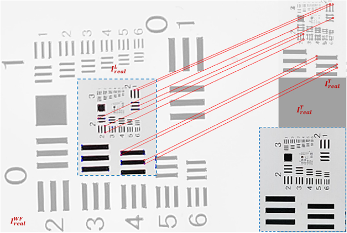
Schematic of the zoom-based dataset production
6, short-focus image (IrealWF) and GT image (IrealT) can be captured in BMP format, as pairs. Given a short-focus image (IrealWF) and long-focus image (IrealT), we first extract the feature points of the images to be matched, represented by the blue circles. Then the brute force matching method is utilized to obtain a preregistration feature point pair, represented by the red lines.
-
(2) Random Sample Consensus (RANSAC algorithm) [55] is an iterative algorithm. In each iteration, the curve is fitted by randomly selecting sample points, finding the sample points whose distance from the fitted curve is within the tolerance range and counting the number, and then entering the next iteration until the limit of cycle times is reached. In this work, RANSAC is used to calculate the homography matrix to convert the homography transformation from GT image to low-resolution (LR) image (IrealL). The calculation method can be described as:
$$\left[\begin{array}{c}x\mathrm{^{\prime}}\\ y\mathrm{^{\prime}}\\ 1\end{array}\right]=\left[\begin{array}{cc}R& T\\ {0}^{T}& 1\end{array}\right]\left[\begin{array}{c}x\\ y\\ 1\end{array}\right]$$(3)where (x', y') and (x, y) are the key coordinates of the target image and the source image, respectively. R is the rotation matrix and T is the translation matrix.
-
(3) We calculate the relationship to find the LR image corresponding to the GT image and save it. For non-standard image pairs, a uniform aspect ratio (4) is also required. Final obtainable pairs (LR, GT) are sent to the network for training (100 pairs) until the trained model achieves reliable results.

Appendix 2
Image formation strategy
The image formation process is on the basis of compositing a panorama from a set of narrow-field images. In our strategy, the overlapping requirement of stitched FOV is removed comparing with the conventional systems. The advantage for the DLBP camera, is that the calibration operation can be achieved once the position and optical parameters of each camera are predicted. Benefiting from independent cameras, the stitching robustness is no longer restricted by texture information. The most important point is that the saved FOV can focus on covering richer information, which dramatically reduces the hardware cost and simplifies the system.
Image formation strategy, as a scalable and parallelizable solution that exploits the multiscale features provided by the DLBP camera, which is amenable for GPU architecture. Parallel computing can be handled by CUDA interface [56]. GPU thread T is the basic processing unit, as contained in a Block structure. As depicted in Fig.

Schematic of the thread organization of parallel pixel mapping. The black pixels represent the final composite space, here the composite space is divided into multiple blocks comprising of CUDA threads, and each input pixel is executed by a CUDA thread which transforms the coordinate system of that pixel
7, each input pixel is executed by a CUDA thread which transforms the coordinate system of that pixel and is mapped to the composite space. The whole FOV is stitched by multiple sub-FOVs, which is conducive to parallelization. The pixel-thread relationship that participates in the calculation is defined as:
where W and H denote the number of the horizontal and the vertical pixels of the image, respectively, and M and N denote the number of the created horizontal Blocks and vertical Blocks, respectively. Once the calibration of the camera is implemented, we will build a set of matrices {H#} for successive stitching, which transforms the local pixels to the composite pixels. The final composite image is computed as follows:
here \(\left[\begin{array}{c}x\\ y\\ 1\end{array}\right]\)# denotes the coordinate of the input pixel, # is the serial number in each camera. An interactive example can be executed over the stitched-FOV using the SR model with computational zoom.
The requirements of different application scenarios/distance may lead to a fundamental compromise between accuracy and efficiency. In fact, the seam line/exposure and the imaging speed are relative consideration for the final composite panorama because the DLBP operates on an ordinary computer. However, the stitching matrix is different and could be fine-tuned according to the requirements of the application scenario/distance because the mapping matrix is not easy to establish, faced with a compromise between accuracy and speed. Our pipeline should not only take into account the real-time efficiency of the project, but also eliminate it as much as possible, which is a choice to weigh the pros and cons. For a stitched example in Fig.

Image formation example with seamless stitching. a-f Sub images captured using DLBP camera. g Stitched-seamless panorama composited using 6 sub-images (a-f)
8, each sub image (a-f) is captured using our proposed DLBP, which has different exposure and seams because of the complex real-world environment. The pipeline may place more emphasis on exposure and stitching phenomena, and a more complex matrix will be created at this time. As illustrated in Fig. 8(g), the dark cloud of that varies from the right to the left in the sky and returns to the roof of the building. The stitched-seamless panorama effectively eliminates the seam lines and exposure differences. In addition, the straight rope is clearly recorded in the FOV of DLBP, here the seamless stitching is favorable to the visual senses.
Appendix 3
Interactive panorama example in the infrared band
We also explore the impact of our strategy on infrared-panoramic SR imaging, as illustrated in Fig.

Interactive panorama example in the infrared band, covering 0.3–4 km. a Infrared panorama captured using the DLBP camera, which is stitched by 6 sub-images. b-e Infrared-SR reconstruction images with 4 × computational zoom, which is one-to-one corresponding to the label area in Fig. 9a
9. The infrared panorama (Fig. 9a) depicts the whole downtown Chengdu at 10 p.m, captured using the DLBP camera with 30 MPs. Supplementary Movie S3 is an interactive panorama example with SR and 4 × computational zoom in the infrared band, operates at 30 fps. The images (Figs. 9b-e) are cropped from the video frames. As illustrated in Fig. 9b, it provides specific details, such as exactly how many cars (5) are waiting for traffic lights near the zebra crossing, and exactly how many zebra crossings (21) are located on the road over the stitched FOV. Here the lights of the vehicle group come together to cause local overexposure. Figure 9c shows that our strategy continues to perform well in response to long-range and ultra-depth-of-field (DOF) demands, for instance, the layering between each tall building in the distance (4 km) is palpable. The brightness of this scene in Fig. 9d varies from the regions of bright street to the areas of deep shadow, which provides the information of high-dynamic-range street. Figure 9e also provides details, such as exactly how many floors (9) are located in the cropped FOV from infrared panorama.
Appendix 4
Crowd identification and tracking module
Observation of group activity has become one of the research hotspots of wide-FOV cameras with high-resolution. The video sequences in Fig.

Crowd tracking on live broadcast of sports events. a-f Video frames at different instant, where basketball players in motion are tracked and represented by yellow rectangular boxes, which helps us to further observe social group activities
10 are captured at different instant using 2 cameras in the DLBP camera because of high altitude control and FOV occlusion. As an example with real time, taken at SCU East Stadium, it reveals the live broadcast of the event of the players who are participating in a basketball match. Here basketball players who are moving are recognized and tracked in real time until they disappear in the field of vision, herein, we envisage that our strategy of enlightening effect on intelligent transportation and group monitoring. A large number of examples are captured to verify our parallel camera. For the crowded scene at SCU East Stadium, a feature recognition algorithm is introduced to detect the human. People on the move are tracked in real time using kernelized correlation filter (KCF), while some people have their backs to the camera, the algorithm works well because basketball players are at a suitable scale. We will continue to enrich our application scenarios and further improve the accuracy rate in future work. The DLBP camera has great potential for live broadcast of large-scene sports events.
Appendix 5
Comparisons of ours with the conventional systems and methods
Our strategy has competitive advantages on improving system complexity, volume and performance. As illustrated in Fig.

Comparison of our system with the conventional system. a Imaging schematic of the conventional zoom strategy. b Imaging schematic of our strategy
11, our strategy has already improved ~ 100 × improvements in zoom speed relative to the conventional systems, such as ours (30 fps) and traditions (3 s +). We believe that this technology can greatly improve the system resolution without any additional hardware on the premise of simplifying the system. We also compare the performance metrics of DLBP camera with the world's most famous parallel cameras (Table S3).
As illustrated in Fig.

12, we also compared the reconstruction of our end-to-end model with the world-famous super-resolution models, from which it can be seen that our reconstruction effect is ahead of other models. From two sets of examples, here our advantage is to resist mosaic phenomenon, and the ability to describe texture details is more prominent due to the addition of attention mechanism. As illustrated in Fig.

Visualization of feature maps in computational model
13, the processing details of the computational model are visualized so that the results can be better evaluated.
Rights and permissions
Open Access This article is licensed under a Creative Commons Attribution 4.0 International License, which permits use, sharing, adaptation, distribution and reproduction in any medium or format, as long as you give appropriate credit to the original author(s) and the source, provide a link to the Creative Commons licence, and indicate if changes were made. The images or other third party material in this article are included in the article's Creative Commons licence, unless indicated otherwise in a credit line to the material. If material is not included in the article's Creative Commons licence and your intended use is not permitted by statutory regulation or exceeds the permitted use, you will need to obtain permission directly from the copyright holder. To view a copy of this licence, visit http://creativecommons.org/licenses/by/4.0/.
About this article

Cite this article
Liu, SB., Xie, BK., Yuan, RY. et al. Deep learning enables parallel camera with enhanced- resolution and computational zoom imaging. PhotoniX 4, 17 (2023). https://doi.org/10.1186/s43074-023-00095-3
Received:
Revised:
Accepted:
Published:
DOI: https://doi.org/10.1186/s43074-023-00095-3